MESOSCALE CONVECTIVE SYSTEM

written by ZAMG

KEY PARAMETERS

As already mentioned in the description of the meteorological physical background, the key parameters have to be divided into those characteristic of the small to mesoscale model of the MCS itself and those characteristic of the synoptic MCS environment (compare meteorological physical background).

Mesoscale conceptual model for MCS

For nearly all conceptual models numerical derived parameters show up as key parameters. In the case of convective developments the key parameters are relevant observations and additional artificial satellite channels. The following material will be used:

• satellite imagery with an appropriate cold cloud top enhancement:
  
  • typical circular and oval shape of the MCS
  • cloud top temperatures below approximately -30° C
  • typical grey shade distribution within the MCS (compare cloud structure in satellite image)
  
  5 August 1998/00 UTC - IR image (enhanced)
  
  
  
  
• weather reports:
  
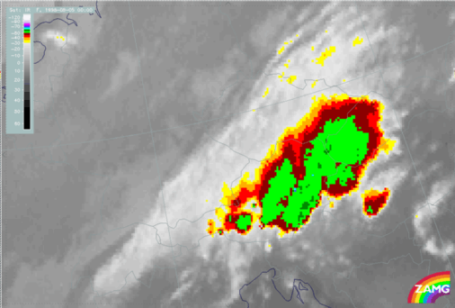
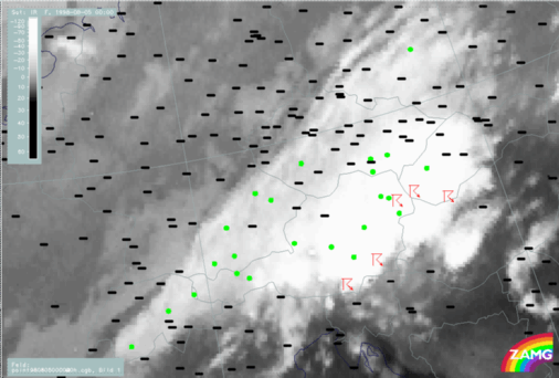
  • Cb, thunderstorms, showers (compare weather reports)
  
  5 August 1998/00 UTC - IR image; symbols: weather events (green: rain and showers, blue: drizzle, cyan: snow, purple: freezing rain, red: thunderstorm with precipitation, orange: hail, black: no actual precipitation or thunderstorm with precipitation)
  
  
  
  
• lightning reports:
  
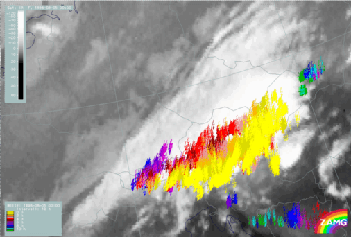
  5 August 1998/00 UTC - IR image; symbols: sferics
  
  
  
  
• radiosonde station analysis:
  
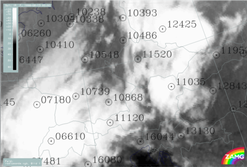
  13 August 1998/00 UTC - IR image; location of radiosonde stations
  
  
  
  
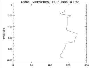
  • wind profile
    The wind direction in the lower and mid-levels of the troposphere, especially in front of and within the area of the right leading edge of the cell, is characterized by a turning to the right with height.
    
    13 August 1998/00 UTC - radiosonde station Munich; wind direction
    
    
    
    
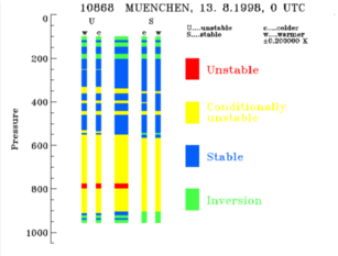
  • stability analysis
    
    13 August 1998/00 UTC - radiosonde station Munich; column: stability analysis (blue: absolutely stable, yellow: conditionally unstable, red: absolutely unstable, green: inversion)
    
  
  
  
• development images indicating new development or decay of cloudiness:
  a typical life cycle can be detected in the development images (compare also the chapter SATELLITE CHANNELS USED IN THE MANUAL channel combinations and artifical channels ):
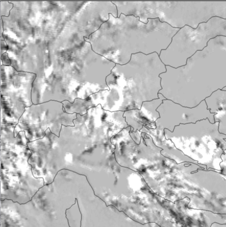
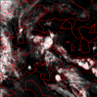
  • developing stage: nearly the whole MCS cloudiness in the IR appears as a white area in the development image, indicating newly developed cloud pixels.
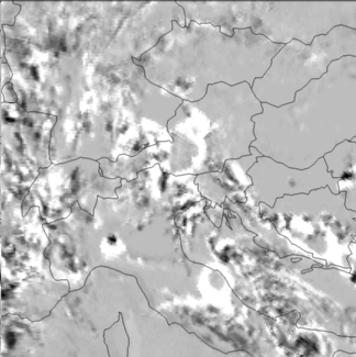
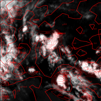
  • mature stage: the biggest area of MCS cloudiness in the IR is a grey area in the development image, indicating no strong further development and not yet any decay; in this stage only the MCS boundaries show white signals in the development image, revealing a typical circular to oval shape of grey areas surrounded by white circles.
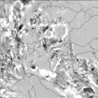
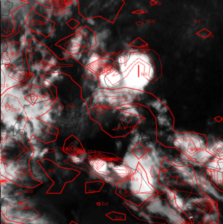
  • dissipating stage: black areas develop mostly at the rearward edges initially but late ron black areas develop at several areas within the whole MCS.
  
  
  Left: 5 June 1998/13 - 14 UTC - IR development image
  Right: 5 June 1998/14 UTC - IR image; lines: red: mean values of grey shades of cloud development and decay
  

  
  Left: 5 June 1998/14 - 15 UTC - IR development image
  Right: 5 June 1998/15 UTC - IR image; lines: red: mean values of grey shades of cloud development and decay
  

  
  Left: 5 June 1998/17 - 18 UTC - IR development image
  Right: 5 June 1998/18 UTC - IR image; lines: red: mean values of grey shades of cloud development and decay
  

  The brightest values in the development image can be found at the stage when completely new cloudiness develops; if the tops within an already existing MCS become colder, or a sub-cell within the MCS grows to produce colder tops, the development image shows only light grey shades. In these cases also the features themselves have to be observed as they show the circular pattern of the rising sub-cell.
  
  The investigation of development images is promising but relatively new, and consequently they have still to be studied and tested in more detail.
  
  

• Radar (written by FMI):
  Another very prominent observation tool is radar (compare meteorological physical background). Although this manual concentrates on satellite imagery, the following provides an introduction to radar. More details may be found in relevant radar literature. One important fact is that with radar small scale features within the MCS at different heights can be observed.
  
  The following paragraphs introduce and illustrate different radar reflectivity products:
  
  
  • Plain Position Indication (PPI)
    One elevation (usually close to zero), all azimuths. PPI is the fastest of all radar products and therefore suitable for studying the fast-developing mesoscale storms.
  • Constant Altitude Plain Position Indication (CAPPI)
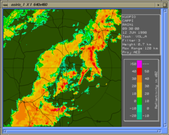
    Traditional PPI has two problem areas: near the radar site there is often ground clutter. In the lowest beam PPI clutter is often so strong that filtering removes also the weather signals (a gap in the middle). Secondly, far from the radar source the beam overshoots precipitation, partly or totally. CAPPI is an attempt to avoid the problems of PPI. Constant altitude data are picked and interpolated from different elevation scans. Practically, beyond a certain distance, the lowest available data are picked and the result is called PseudoCAPPI.
    
    
    
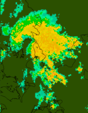
  • Echo Top
    Echo top is the tool to follow a developing convective system. Use together with temperature profile. When tops reach -15, precipitation begins, when tops reach -25, the chance of for thunder is considerable.
    
    
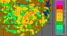
    Some towering tops (in red) rise above a more widespread cloud mass. These are embedded cumulonimbus towers.
  • MAX
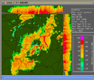
    MAX is the tool to identify the strongest cells in a multicell system. This is essential e.g. for aviation briefing. High dBZ values at higher altitudes (e.g. +30 dBZ at 5 kilometres) almost certainly relate to wet graupel or hail, and indicate strong updrafts.

    These two images are from the same moment as the cross sections below (east and north from the centre). Note in the MAX image the additional information about the vertical structure of the cells, provided by the side panels.

  
  
  
  • Range Height Indicator (RHI)
    RHI or cross section is not the primary tool, but once you have identified a possible MCS, a good cross section helps you to study the vertical structure and to identify the possible hail-generating cells.
    
    
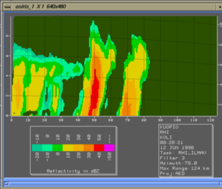
    Here is a cross section through several Cumulonimbus cells, one of which is stronger than the others. Note that weak intensities in the thinner parts of the anvil (below -10 dBZ) can only be detected close to the radar (left part of the image).
    
    
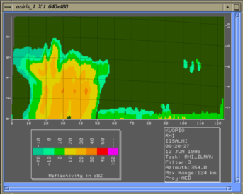
    The bright band (maximum reflectivity layer due to melting hydrometeors near 0 degree isotherm) can be detected even in convective rain, even though, due to strong vertical movements, it is not always as clear as in stratiform rain.
  • Accumulated precipitation for n hours (RAINN product)
    One of the typical questions after an MCS has stormed over an area is "How many millimetres ?" Gauge measurements are quite accurate (despite wind-induced error!) but the synoptic network is rather sparse - and often you have to wait until 06 UTC or 18 UTC to get the readings. Radar products for Accumulated precipitation are less accurate, but they have outstanding resolution both in space and time. They are generated from CAPPIs, so all error sources for CAPPIs are present here. Remember that far from the radar source the measurement bin is quite big and well above the ground! For a radar RAINN product, it is often safest (in press interviews etc.) to:
    • point out the areas of maximum precipitation
    • give the millimetres assuming 50% accuracy (so "about one", "less than five", "20 - 30 mm" are quite safe phrases).
    
    
    
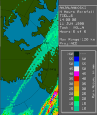
    A small but intense shower gave flash flooding in a limited area - impossible to be detected by any other instrument than radar! However, the absolute maximum values (over 60 millimetres in six hours) must be suspect here, as hail was present. The striped structure of the precipitation area is due to movement of Cb cells between the individual CAPPIs which have been used as raw material in this composite.
  • Doppler winds
    A doppler radar can be used to determine wind speed from that of echo-giving droplets. A classical Doppler wind PPI is difficult to interpret without wide experience. A well-formed mesocyclone can be detected by a Doppler radar as a couplet in the velocity data, which indicates a circulation (motion away and towards the radar). The couplet is most typical for tornadic supercells and other intense twisters. Nowadays the data are often displayed as more sophisticated wind products.
    
    
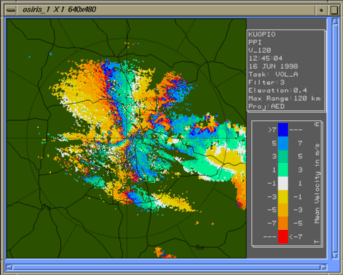
    Doppler speed as measured (wind component parallel to radar beam). Blue and green is away from radar, red and orange towards radar. Ambigous speed scale is too small so the colours have to beu interpreted carefully (white is zero or eight or fifteen).
    
    
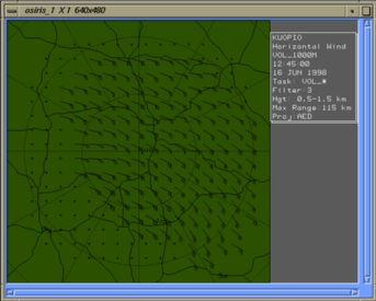
    The same information as in image above, interpreted to standard wind arrows. As each arrow is averaged from a relatively large slice, small phenomena like tornadoes are likely to be filtered out.
  • Time - Height cross section of VVP wind profiles (THVVP - time series of wind profiles)
    The tool to study changes in wind shear. This is the best mesoscale tool for it, given enough time resolution (typically a new sounding every 15 or 30 minuntes). Remember that radar winds always represent an average of a larger volume, e.g.in this case a cylinder 40 kilometres in radius, 200 metres thick. If the wind field is not linear, the average through such a volume can be erroneus. Suspect non-continous winds.
    
    
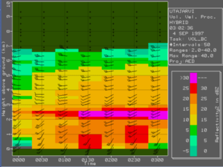
    Time as x-coordinate, height as y-coordinate. Coloured background is averaged reflectivity in a cylinder with 40 kilometres radius around the radar. Wind barbs averaged in the same cylinder. Note the wind shear near ground due to Ekman spiral and warm advection, and reflectivity maximum near 2.5 kilometres due to bright band (melting layer) after 01:00 UTC. (This example is not from an MCS case, but a more stratiform precipitation, first snow, later rain.)

    Vertical velocity sounds like a good idea, but you cannot distinguish the speed of falling droplets from the speed of rising or sinking air parcels, so if you study this put more emphasis on changes to this parameter than the actual values. (Vertical velocity can be used instead of reflectivity in the THVVP. Another possible parameter is divergence/convergence.)

Meso- to synoptic scale conceptual models of the synoptic environment of MCSs

For the larger scale of the synoptic environment numerical parameters can be used as key parameters:

• Stability index on isobaric surfaces:
  In this manual the Showalter Index is used. The relevant area should be indicated as an area with high probability for Cb development; in the case of the Showalter index values below 3 units are expected.
  
  5 June 1998/18 UTC - IR image; lines: yellow: Showalter index 500/850 hPa
  
  
  
  
• Numerical model parameters on isobaric surfaces:
  special attention is paid to:
  • front and thickness ridge indicating parameters (TFP, equivalent thickness, TA): the typical configurations for fronts and thickness ridge are described in detail for the relevant conceptual models (compare also chapters of COLD FRONT CF CC CW SF AC , WARM FRONT WB WS WF and OCCLUSION OC IO CC CD BB ).
    
    24 August 1997/18 UTC - IR image; lines: blue: thermal front parameter (TFP) 500/850 hPa, green: equivalent thickness 500/850 hPa, yellow: Showalter index 500/850 hPa
    

  • Equivalent potential temperature at 850 hPa:
    tongue of high values of THETA_E; MCS develop in the area of the maximal values
    
    24 August 1997/18 UTC - IR image; lines: blue: thermal front parameter (TFP) 500/850 hPa, magenta: equivalent potential temperature at 850 hPa
    

• Numerical model parameters in vertical cross section:
  This part will be described in more detail in the chapter on the vertical cross sections (compare appearance in vertical cross section). Special attention is paid to:
  • behaviour of isentropes
  • temperature advection
  • convergence
• Relative streams for discrimination of different air masses:
  special attention is paid to: vertical distribution of relative streams: a warm moist conveyor belt like the warm conveyor belt in low to middle layers, and a cold dry conveyor belt like the dry intrusion above (compare meteorological physical background).
  
  

The conceptual models of typical synoptic environments can be detected rather easily; they contain the signal that in these areas there is a high probability for the development of MCSs. But it is not possible to determine where within this bigger area the much smaller MCSs will develop. So once a typical MCS environment is located the only possibility is to start intensive observations; after having detected the initial stage of a convective cell two approaches may be followed:

• the use of the small scale MCS conceptual model for forecasting development and weather activity
• the displacement of the MCS with nowcasting methods

HELP - I AM LOST

MAIN MENU OF THE MANUAL

SUB-MENU OF THE MESOSCALE CONVECTIVE SYSTEM

SECOND SUB-CHAPTER - METEOROLOGICAL PHYSICAL BACKGROUND

FOURTH SUB-CHAPTER - WEATHER EVENTS